Examples
Example 01: Calculation of free energy
In this example, a simple calculation of the Helmholtz free energy $F(NVT)$ is illustrated. We use a Fe BCC structure at 100K.
The EAM potential that will be used: Meyer, R, and P Entel. “Martensite-austenite transition and phonon dispersion curves of Fe1−xNix studied by molecular-dynamics simulations.” Phys. Rev. B 57, 5140.
The reference data is from: Freitas, Rodrigo, Mark Asta, and Maurice de Koning. “Nonequilibrium Free-Energy Calculation of Solids Using LAMMPS.” Computational Materials Science 112 (February 2016): 333–41.
Solid free energy
The input file for calculation of solid BCC Fe at 100 K is provided in the folder. A detailed description of the input file is available here. The calculation can be started from the terminal using:
calphy -i input.yaml
This should give a message:
Total number of 1 calculations found
calphy is running in the background executing the calculation. A new folder called fe-BCC-100-0, and files called fe-BCC-100-0.sub.err and fe-BCC-100-0.sub.out will also be created.
After the calculation is over, the results are available in the report.yaml file. The file is shown below:
average:
  spring_constant: '3.32'
  vol/atom: 11.994539429692749
input:
  concentration: '1'
  element: Fe
  lattice: bcc
  pressure: 0.0
  temperature: 100
results:
  error: 0.0
  free_energy: -4.263568357143783
  pv: 0.0
  reference_system: 0.015029873513789175
  work: -4.278598230657573
The calculated free energy is $-4.2636$ eV/atom, the value reported in the publication is $-4.2631147(1)$ eV/atom. The calculated value can be further improved by increasing the system size, and by increasing the switching time.
Example 02: Phase transformation in Fe
In this example, we will make use of the temperature sweep algorithm in calphy to calculate the transformation temperature for BCC to FCC transition in Fe.
The EAM potential that will be used: Meyer, R, and P Entel. “Martensite-austenite transition and phonon dispersion curves of Fe1−xNix studied by molecular-dynamics simulations.” Phys. Rev. B 57, 5140.
The reference data is from: Freitas, Rodrigo, Mark Asta, and Maurice de Koning. “Nonequilibrium Free-Energy Calculation of Solids Using LAMMPS.” Computational Materials Science 112 (February 2016): 333–41.
The input file is provided in the folder. The calculation can be started from the terminal using:
calphy -i input.yaml
In the input file, the calculations block is as shown below:
- mode: ts
  temperature: [100, 1400]
  pressure: [0]
  lattice: [BCC]
  repeat: [5, 5, 5]
  state: [solid]
  nsims: 1
- mode: ts
  temperature: [100, 1400]
  pressure: [0]
  lattice: [FCC]
  repeat: [5, 5, 5]
  state: [solid]
  nsims: 1
  lattice_constant: [6.00]
The mode is listed as ts, which stands for temperature sweep. The sweep starts from the first value in the temperature option, which is 100 K. The free energy is integrated until 1400 K, which is the second value listed. Furthermore, there are also two calculation blocks. You can see that the lattice mentioned is different; one set is for BCC structure, while the other is FCC.
Once the calculation is over, there will a file called temperature_sweep.dat in each of the folders. This file indicates the variation of free energy with the temperature. We can read in the files and calculate the transition temperature as follows:
import numpy as np

bt, bfe, bferr = np.loadtxt("ts-BCC-100-0/temperature_sweep.dat", unpack=True)
ft, ffe, fferr = np.loadtxt("ts-FCC-100-0/temperature_sweep.dat", unpack=True)

args = np.argsort(np.abs(bfe-ffe))
print(bt[args[0]], "K")

plt.plot(bt, bfe, color="#E53935", label="bcc")
plt.plot(ft, ffe, color="#0097A7", label="fcc")
plt.xlabel("Temperature (K)", fontsize=12)
plt.ylabel("F (ev/atom)", fontsize=12)
plt.legend()
![]()
A jupyter notebook that calculates the transition temperature is shown here.
Example 03: Calculation of Cu melting temperature
In this example, the melting temperature for Cu is calculated using a combination of free energy calculation and temperature sweep.
The EAM potential we will use is : Mishin, Y., M. J. Mehl, D. A. Papaconstantopoulos, A. F. Voter, and J. D. Kress. “Structural Stability and Lattice Defects in Copper: Ab Initio , Tight-Binding, and Embedded-Atom Calculations.” Physical Review B 63, no. 22 (May 21, 2001): 224106.
The calculation block gives the input conditions at which the calculation is carried out. First of all, the mode is ts, a temperature sweep over the temperature range given in the temperature keyword will be done. FCC and LQD lattice are chosen, the former for solid and the latter for liquid. The potential file is specified in pair_coeff command in the md block.
The calculation can be run by,
calphy -i input.yaml
Once submitted, it should give a message Total number of 2 calculations found. It will also create a set of folders with the names mode-lattice-temperature-pressure. In this case, there will be ts-FCC-1200-0 and ts-LQD-1200-0. If there are any errors in the calculation, it will be recoreded in ts-FCC-1200-0.sub.err and ts-LQD-1200-0.sub.err. Once the calculation starts, a log file called tint.log will be created in the aforementioned folders. For example, the tint.log file in ts-FCC-1200-0 is shown below:
2021-07-08 15:12:02,873 calphy.helpers INFO     At count 1 mean pressure is -5.337803 with 12.625936 vol/atom
2021-07-08 15:12:09,592 calphy.helpers INFO     At count 2 mean pressure is -5.977502 with 12.625639 vol/atom
2021-07-08 15:12:15,790 calphy.helpers INFO     At count 3 mean pressure is -6.557647 with 12.623906 vol/atom
2021-07-08 15:12:22,059 calphy.helpers INFO     At count 4 mean pressure is -2.755662 with 12.624017 vol/atom
2021-07-08 15:12:28,157 calphy.helpers INFO     At count 5 mean pressure is -1.306381 with 12.625061 vol/atom
2021-07-08 15:12:34,405 calphy.helpers INFO     At count 6 mean pressure is 0.718567 with 12.625150 vol/atom
2021-07-08 15:12:40,595 calphy.helpers INFO     At count 7 mean pressure is 2.185729 with 12.625295 vol/atom
2021-07-08 15:12:47,020 calphy.helpers INFO     At count 8 mean pressure is 2.162312 with 12.625414 vol/atom
2021-07-08 15:12:53,323 calphy.helpers INFO     At count 9 mean pressure is 1.137092 with 12.624953 vol/atom
2021-07-08 15:12:59,692 calphy.helpers INFO     At count 10 mean pressure is 0.377612 with 12.625385 vol/atom
2021-07-08 15:12:59,693 calphy.helpers INFO     finalized vol/atom 12.625385 at pressure 0.377612
2021-07-08 15:12:59,693 calphy.helpers INFO     Avg box dimensions x: 18.483000, y: 18.483000, z:18.483000
2021-07-08 15:13:05,878 calphy.helpers INFO     At count 1 mean k is 1.413201 std is 0.072135
2021-07-08 15:13:12,088 calphy.helpers INFO     At count 2 mean k is 1.398951 std is 0.065801
2021-07-08 15:13:12,090 calphy.helpers INFO     finalized sprint constants
2021-07-08 15:13:12,090 calphy.helpers INFO     [1.4]
The file gives some information about the preparation stage. It can be seen that at loop 10, the pressure is converged and very close to the 0 value we specified in the input file. After the pressure is converged, box dimensions are fixed, and the spring constants for the Einstein crystal are calculated.
The ts mode consists of two stages, the first step is the calculation of free energy at 1200 K, followed by a sweep until 1400 K. The results of the free energy calculation is recorded in report.yaml file. The file is shown below:
average:
  spring_constant: '1.4'
  vol/atom: 12.625384980886036
input:
  concentration: '1'
  element: Cu
  lattice: fcc
  pressure: 0.0
  temperature: 1200
results:
  error: 0.0
  free_energy: -4.071606995367944
  pv: 0.0
  reference_system: -0.7401785806445611
  work: -3.331428414723382
In the file, the average and input quantities are recorded. The more interesting block is the results block. Here the calculated free energy value in eV/atom is given in the free_energy key. The free energy of the reference system is given in reference_system and the work done in switching is under work. The error key gives the error in the calculation. In this case, its 0 as we ran only a single loop (see nsims). The report.yaml file for liquid looks somewhat similar.
average:
  density: 0.075597559457131
  vol/atom: 13.227983329718013
input:
  concentration: '1'
  element: Cu
  lattice: fcc
  pressure: 0.0
  temperature: 1200
results:
  error: 0.0
  free_energy: -4.058226884054426
  pv: 0.0
  reference_system: 0.6852066332000204
  work: 4.743433517254447
The main difference here is that under the average block, the density is reported instead of spring_constant.
The variation of the free energy within the temperature range is given in the temperature_sweep.dat files instead of each of the folders. The file contains three columns, temperature, free energy and the error in free energy. The files are read in and plotted below.
import numpy as np
import matplotlib.pyplot as plt

st, sfe, sferr = np.loadtxt("ts-FCC-1200-0/temperature_sweep.dat", unpack=True)
lt, lfe, lferr = np.loadtxt("ts-LQD-1200-0/temperature_sweep.dat", unpack=True)

plt.plot(st, sfe, color="#E53935", label="solid")
plt.plot(lt, lfe, color="#0097A7", label="liquid")
plt.xlabel("Temperature (K)", fontsize=12)
plt.ylabel("F (ev/atom)", fontsize=12)
plt.legend()
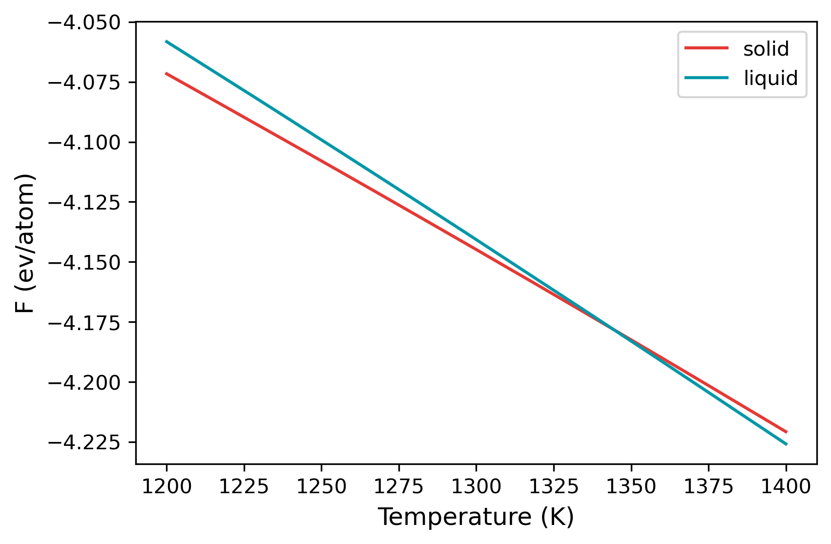
From the plot, at temperatures below 1300 K, solid is the more stable structure with lower free energy. Around 1340 K, liquid becomes the more stable structure. We can find the temperature at which the free energy of both phases are equal, which is the melting temperature.
args = np.argsort(np.abs(sfe-lfe))
print(st[args[0]], "K")
Example 04: Pressure-temperature phase diagram of Cu
In this example, the pressure-temperature phase diagram of Cu will be calculated.
The EAM potential we will use is : Mishin, Y., M. J. Mehl, D. A. Papaconstantopoulos, A. F. Voter, and J. D. Kress. “Structural Stability and Lattice Defects in Copper: Ab Initio , Tight-Binding, and Embedded-Atom Calculations.” Physical Review B 63, no. 22 (May 21, 2001): 224106.
The input file is provided in the folder. The calculation is very similar to the calculation of melting temperature. However, we calculate the melting temperature for various pressures to arrive at the phase-diagram.
There are five input files in the folder, from input1.yaml to input5.yaml. Each file contains the calculations for a single pressure. You can also add all of the calculations in a single file under the calculations block. It is split here into five files for the easiness of running the calculations on relatively small machines.
The calculation can be run by:
calphy -i input1.yaml
and so on until input5.yaml. After the calculations are over, we can read in the results and compare it.
import numpy as np
import matplotlib.pyplot as plt
The starting temperatures and pressures for our calculations:
temp = [1600, 2700, 3700, 4600]
press = [100000, 500000, 1000000, 1500000]
Now a small loop which goes over each folder and calculates the melting temperature value:
tms = []

for t, p in zip(temp, press):
    sfile =  "ts-FCC-%d-%d/temperature_sweep.dat"%(t, p)
    lfile =  "ts-LQD-%d-%d/temperature_sweep.dat"%(t, p)
    t, f, fe = np.loadtxt(sfile, unpack=True)
    t, l, fe = np.loadtxt(lfile, unpack=True)
    args = np.argsort(np.abs(f-l))

    tms.append(t[args[0]])
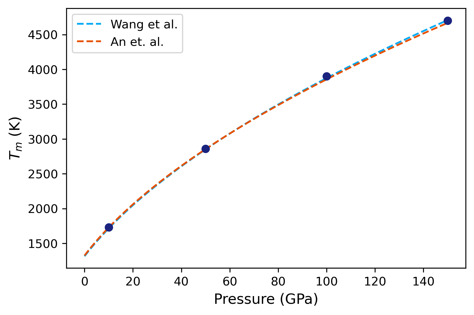
To compare our results, we will use a Simon equation, given by,
We will use reported values for parameters \(T_{m0}\), \(a\) and \(b\) from two different publications:
def get_tm(press):
    tm = 1315*(press/15.84 + 1)**0.543
    return tm
def get_tm2(press):
    tm = 1325*(press/15.37 + 1)**0.53
    return tm
An array for pressures over which the two equations will be fit, and values of the two expressions are calculated.
pfit = np.arange(0, 151, 1)
tma = get_tm(pfit)
tmb = get_tm2(pfit)
plt.plot(pfit, tma, ls="dashed", label="Wang et al.", color="#03A9F4")
plt.plot(pfit, tmb, ls="dashed", label="An et. al.", color="#E65100")
plt.plot(np.array(press)/10000, tms, 'o', color="#1A237E")
plt.xlabel("Pressure (GPa)", fontsize=12)
plt.ylabel(r"$T_m$ (K)", fontsize=12)
plt.legend()
The analysis code can be found in this notebook.