Example 09: Pressure scaling#
In some cases, it is useful to obtain the free energy as a function of the pressure. The calphy mode pscale allows to do this.
The EAM potential we will use is : Mishin, Y., M. J. Mehl, D. A. Papaconstantopoulos, A. F. Voter, and J. D. Kress. “Structural Stability and Lattice Defects in Copper: Ab Initio , Tight-Binding, and Embedded-Atom Calculations.” Physical Review B 63, no. 22 (May 21, 2001): 224106.
The input file is provided in the folder. The pressure scale input file is input2.yaml, in which we calculate the free energy at 1200 K from 0 to 1 GPa. To compare, we do direct free energy calculations at the same temperature and pressures of 0, 0.5 and 1 GPa. The input for this is provided in input1.yaml.
The calculation can be run by:
calphy -i input1.yaml
calphy -i input2.yaml
After the calculations are over, we can read in and analyse the results.
[1]:
import numpy as np
import matplotlib.pyplot as plt
[2]:
p1 = [0, 5000, 10000]
fe1 = [-4.072, -4.032, -3.993]
The above values are taken from the report.yaml files in the corresponding folders.
Note that calphy uses bar as the unit of pressure.
Now read in the pressure scaling results.
[5]:
p2, fe2, ferr2 = np.loadtxt("pscale-FCC-1200-0/pressure_sweep.dat", unpack=True)
Now plot
[6]:
plt.plot(p2, fe2, color="#E53935", label="pscale")
plt.plot(p1, fe1, 'o', color="#0097A7", label="direct")
plt.xlabel("Pressure (bar)", fontsize=12)
plt.ylabel("F (ev/atom)", fontsize=12)
plt.legend()
[6]:
<matplotlib.legend.Legend at 0x7fe37731d0c0>
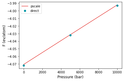
There is excellent agreement between direct calculations and pressure scaling. Now we can also do the calculations for a pressure range of 1-2 GPa. The input is given in input3.yaml and input4.yaml for the pressure scaling and direct calculations respectively.
[49]:
p3 = [10000, 15000, 20000]
fe3 = [-3.994, -3.955, -3.916]
[50]:
p4, fe4, ferr4 = np.loadtxt("pscale-FCC-1200-10000/pressure_sweep.dat", unpack=True)
[52]:
plt.plot(p4, fe4, color="#E53935", label="pscale")
plt.plot(p3, fe3, 'o', color="#0097A7", label="direct")
plt.xlabel("Pressure (bar)", fontsize=12)
plt.ylabel("F (ev/atom)", fontsize=12)
plt.legend()
[52]:
<matplotlib.legend.Legend at 0x7f71512557b0>
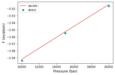
Once again, for the higher pressure interval, there is excellent agreement between the two methods.