Example 03: Manual calculation of Cu melting temperature

In this example, the melting temperature for Cu is calculated using a combination of free energy calculation and temperature sweep.

The EAM potential we will use is : Mishin, Y., M. J. Mehl, D. A. Papaconstantopoulos, A. F. Voter, and J. D. Kress. “Structural Stability and Lattice Defects in Copper: Ab Initio , Tight-Binding, and Embedded-Atom Calculations.” Physical Review B 63, no. 22 (May 21, 2001): 224106.

The calculation block gives the input conditions at which the calculation is carried out. First of all, the mode is ts, a temperature sweep over the temperature range given in the temperature keyword will be done. fcc lattice are chosen for both calculations, the former with reference phase solid and the latter with the reference phase liquid. The potential file is specified in pair_coeff command in the md block.

The calculation can be run by,

calphy -i input.yaml

Once submitted, it should give a message Total number of 2 calculations found. It will also create a set of folders with the names mode-lattice-referencephase-temperature-pressure. In this case, there will be ts-fcc-solid-1200-0 and ts-fcc-liquid-1200-0. If there are any errors in the calculation, it will be recoreded in ts-fcc-solid-1200-0.sub.err and ts-fcc-liquid-1200-0.sub.err. Once the calculation starts, a log file called calphy.log will be created in the aforementioned folders. The file gives some information about the preparation stage.

The ts mode consists of two stages, the first step is the calculation of free energy at 1200 K, followed by a sweep until 1400 K. The results of the free energy calculation is recorded in report.yaml file. The file is shown below:

average:
  density: 0.07557340045029688
  vol_atom: 13.2345681628356
input:
  concentration: '1.0'
  element: Cu
  lattice: fcc
  pressure: 0.0
  temperature: 1200
results:
  error: 0.0
  free_energy: -4.058705625895811
  pv: 0.0
  reference_system: 1.9111881193348468
  unit: eV/atom
  work: 4.742856409041955

In the file, the average and input quantities are recorded. The more interesting block is the results block. Here the calculated free energy value in eV/atom is given in the free_energy key. The free energy of the reference system is given in reference_system and the work done in switching is under work. The error key gives the error in the calculation. In this case, its 0 as we ran only a single loop (see n_iterations).

The variation of the free energy within the temperature range is given in the temperature_sweep.dat files instead of each of the folders. The file contains three columns, temperature, free energy and the error in free energy. The files are read in and plotted below.

import numpy as np
import matplotlib.pyplot as plt

st, sfe, sferr = np.loadtxt("ts-fcc-solid-1200-0/temperature_sweep.dat", unpack=True)
lt, lfe, lferr = np.loadtxt("ts-fcc-liquid-1200-0/temperature_sweep.dat", unpack=True)

plt.plot(st, sfe, color="#E53935", label="solid")
plt.plot(lt, lfe, color="#0097A7", label="liquid")
plt.xlabel("Temperature (K)", fontsize=12)
plt.ylabel("F (ev/atom)", fontsize=12)
plt.legend()
plt.savefig("tm.png", dpi=300, bbox_inches="tight")

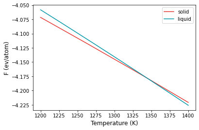
From the plot, at temperatures below 1300 K, solid is the more stable structure with lower free energy. Around 1340 K, liquid becomes the more stable structure. We can find the temperature at which the free energy of both phases are equal, which is the melting temperature.

args = np.argsort(np.abs(sfe-lfe))
print(st[args[0]], "K")

1344.3095672974282 K