Example 12: Calculation of specific heat

In this example, the specific hear for Cu is calculated using a combination of free energy calculation and temperature sweep.

The EAM potential we will use is : Mishin, Y., M. J. Mehl, D. A. Papaconstantopoulos, A. F. Voter, and J. D. Kress. “Structural Stability and Lattice Defects in Copper: Ab Initio , Tight-Binding, and Embedded-Atom Calculations.” Physical Review B 63, no. 22 (May 21, 2001): 224106.

The calculation block gives the input conditions at which the calculation is carried out. First of all, the mode is ts, a temperature sweep over the temperature range given in the temperature keyword will be done.

The calculation can be run by,

calphy -i input.yaml

calculation. In this case, its 0 as we ran only a single loop (see n_iterations).

The variation of the free energy within the temperature range is given in the temperature_sweep.dat files in the simulation folder. The file contains three columns, temperature, free energy and the error in free energy. The files are read in and plotted below.

We start with imports

import numpy as np
import matplotlib.pyplot as plt
import scipy.constants as sc

And some constants which we will use later,

ev_to_j = sc.physical_constants["electron volt-joule relationship"][0]
Av =  sc.physical_constants["Avogadro constant"][0]
A_to_m = 1E-10
kB = sc.physical_constants["Boltzmann constant"][0]

temp, fe, err = np.loadtxt("ts-fcc-solid-400-0/temperature_sweep.dat", unpack=True)

Calculation of \(c_p\) from free energy

The first step is to calculate the entropy from free energy using the following equation,

\[-S = \bigg ( \frac{dF}{dT} \bigg )_V\]

Then differentiating once more provides the specific heat,

\[c_p = T\bigg ( \frac{dS}{dT} \bigg )_p\]

We start by calculating the entropy by taking the gradient, converting it to J/mol K. But before that, we will fit the free energy to a polynomial so that taking gradients is easier. In this case, we will use a fifth order polynomial.

fe_fit_fn = np.polyfit(temp, fe, 5)

Now we take the derivative of the free energy with respect to the temperature.

entropy_fn = -np.polyder(fe_fit_fn, m=1)*ev_to_j/(1/Av)

Now we use this equation:

\[c_p = T\bigg ( \frac{dS}{dT} \bigg )_p\]

to calculate the specific heat

cp_fn = np.polyder(entropy_fn, m=1)

Evaluating this polynomial gives the specific heat

cp_temp = np.polyval(cp_fn, temp)

Note that we calculated:

\[\frac{c_p}{T} = \bigg ( \frac{dS}{dT} \bigg )_p\]

Note the division by \(T\). The reason for this is to reduce the noise in our calculation when comparing with experimental results. Note that if a longer switching time and system size is used, we can use the actual equation. For more details see Fig. 4 in Ref.

In order to compare our results, we plot it together with some experimental values from Ref.

exp_temp = [400, 450, 500, 550, 600, 650, 700, 800,900,1000, 1100, 1200]
exp_cp = [25.25, 25.61, 25.91, 26.21, 26.48, 26.73, 26.99, 27.48, 28.04, 28.66, 29.48, 30.53]

Finally the plot

plt.plot(temp, cp_temp)
plt.plot(exp_temp, np.array(exp_cp)/np.array(exp_temp), 'o')
plt.xlabel("Temperature (K)", fontsize=12)
plt.ylabel(r"$C_p/T$ (J/mol)", fontsize=12)

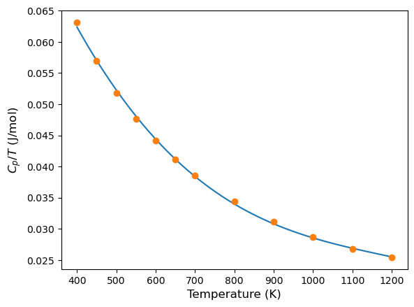
We can see that there is good agreement between the two values.